All Macroscopic Onjects Emit a Continuous

3.1 Atomic Spectra of Gases All Objects Emit Thermal Radiation Characterized by a Continuous Distribution of Wavelengths

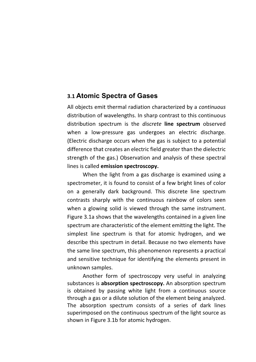
3.1 Atomic Spectra of Gases All objects emit thermal radiation characterized by a continuous distribution of wavelengths. In sharp contrast to this continuous distribution spectrum is the discrete line spectrum observed when a low‐pressure gas undergoes an electric discharge. (Electric discharge occurs when the gas is subject to a potential difference that creates an electric field greater than the dielectric strength of the gas.) Observation and analysis of these spectral lines is called emission spectroscopy. When the light from a gas discharge is examined using a spectrometer, it is found to consist of a few bright lines of color on a generally dark background. This discrete line spectrum contrasts sharply with the continuous rainbow of colors seen when a glowing solid is viewed through the same instrument. Figure 3.1a shows that the wavelengths contained in a given line spectrum are characteristic of the element emitting the light. The simplest line spectrum is that for atomic hydrogen, and we describe this spectrum in detail. Because no two elements have the same line spectrum, this phenomenon represents a practical and sensitive technique for identifying the elements present in unknown samples. Another form of spectroscopy very useful in analyzing substances is absorption spectroscopy. An absorption spectrum is obtained by passing white light from a continuous source through a gas or a dilute solution of the element being analyzed. The absorption spectrum consists of a series of dark lines superimposed on the continuous spectrum of the light source as shown in Figure 3.1b for atomic hydrogen. The absorption spectrum of an element has many practical applications. For example, the continuous spectrum of radiation emitted by the Sun must pass through the cooler gases of the solar atmosphere. The various absorption lines observed in the solar spectrum have been used to identify elements in the solar atmosphere. In early studies of the solar spectrum, experimenters found some lines that did not correspond to any known element. A new element had been discovered! The new element was named helium, after the Greek word for Sun, helios. Helium was subsequently isolated from subterranean gas on the Earth. Using this technique, scientists have examined the light from stars other than our Sun and have never detected elements other than those present on the Earth. Absorption spectroscopy has also been useful in analyzing heavy‐metal contamination of the food chain. For example, the first determination of high levels of mercury in tuna was made with the use of atomic absorption spectroscopy.

Figure 3.1 (a) Emission line spectra for hydrogen, mercury, and neon. (b) The absorption spectrum for hydrogen. Notice that the dark absorption lines occur at the same wavelengths as the hydrogen emission lines in (a).7

7 (K. W. Whitten, R. E. Davis, M. L. Peck, and G. G. Stanley, General Chemistry, 7th ed., Belmont, CA, Brooks/Cole, 2004.) In 1885, a Swiss schoolteacher, Johann Jacob Balmer (1825–1898), found an empirical equation that correctly predicted the wavelengths of four visible emission lines of hydrogen: Hα (red), Hβ (bluegreen), Hγ (blue‐violet), and Hδ (violet). Figure 3.2 shows these and other lines (in the ultraviolet) in the emission spectrum of hydrogen. The four visible lines occur at the wavelengths 656.3 nm, 486.1 nm, 434.1 nm, and 410.2 nm. The complete set of lines is called the Balmer series. The wavelengths of these lines can be described by the following equation, which is a modification made by Johannes Rydberg (1854–1919) of Balmer's original equation: 1  1 1   RH  2  2  n 3, 4, 5, ... 3.1 λ 2 n  where RH is a constant now called the Rydberg constant with a value of 1.0973732 x 107 m–1. The integer values of n from 3 to 6 give the four visible lines from 656.3 nm (red) down to 410.2 nm (violet). Equation 3.1 also describes the ultraviolet spectral lines in the Balmer series if n is carried out beyond n = 6. The series limit is the shortest wavelength in the series and Figure 3.2 The Balmer series of spectral lines for atomic hydrogen, with several lines marked with the wavelength in nanometers. corresponds to n → , with a wavelength of 364.6 nm as in Figure 3.2. The measured spectral lines agree with the empirical equation, Equation 3.1, to within 0.1%. Other lines in the spectrum of hydrogen were found following Balmer's discovery. These spectra are called the Lyman, Paschen, and Brackett series after their discoverers. The wavelengths of the lines in these series can be calculated through the use of the following empirical equations: 1  1   RH1  n 2, 3, 4, ... (3.2) Lymanseries λ  n2  1  1 1   RH 2  2  n 4, 5, 6, ... (3.3) Paschen series λ 3 n  1  1 1   RH   n 5, 6, 7, ... (3.4) Brackett serie s λ 42 n2 

3.2 Early Models of the Atom The model of the atom in the days of Newton was a tiny, hard, indestructible sphere. Although this model provided a good basis for the kinetic theory of gases, new models had to be devised when experiments revealed the electrical nature of atoms. In 1897, J. J. Thomson established the charge‐to‐mass ratio for electrons. The following year, he suggested a model that describes the atom as a region in which positive charge is spread out in space with electrons embedded throughout the region, much like the seeds in a watermelon or raisins in thick pudding (Fig. 3.3). The atom as a whole would then be electrically neutral.

In 1911, Ernest Rutherford (1871–1937) and his students Hans Geiger and Ernest Marsden performed a critical experiment that showed that Thomson's model could not be correct. In this experiment, a beam of positively charged alpha particles (helium nuclei) was projected into a thin metallic foil such as the target in Figure 3.4a. Most of the particles passed through the foil as if it were empty space, but some of the results of the experiment were astounding. Many of the particles deflected from their original direction of travel were scattered through large angles. Some particles were even deflected backward, completely reversing their direction of travel!

Figure 3.3 Thomson's model of the atom. Rutherford explained his astonishing results by developing a new atomic model, one that assumed the positive charge in the atom was concentrated in a region that was small relative to the size of the atom. He called this concentration of positive charge the nucleus of the atom. Any electrons belonging to the atom were assumed to be in the relatively large volume outside the nucleus. To explain why these electrons were not pulled into the

Figure 3.4 (a) Rutherford's technique for observing the scattering of alpha particles from a thin foil target. The source is a naturally occurring radioactive substance, such as radium. (b) Rutherford's planetary model of the atom. nucleus by the attractive electric force, Rutherford modeled them as moving in orbits around the nucleus in the same manner as the planets orbit the Sun (Fig. 3.4b). For this reason, this model is often referred to as the planetary model of the atom. Two basic difficulties exist with Rutherford's planetary model. As we saw in Section 3.1, an atom emits (and absorbs) certain characteristic frequencies of electromagnetic radiation and no others, but the Rutherford model cannot explain this phenomenon. A second difficulty is that Rutherford's electrons are described by the particle in uniform circular motion model; they have a centripetal acceleration. According to Maxwell's theory of electromagnetism, centripetally accelerated charges revolving with frequency f should radiate electromagnetic waves of frequency f. As energy leaves the system, the radius of the electron's orbit steadily decreases (Fig. 3.5). Therefore, as the electron moves closer to the nucleus, the angular speed of the electron will increase, just like the spinning skater. This process leads to an ever‐ increasing frequency of emitted radiation and an ultimate collapse of the atom as the electron plunges into the nucleus. Figure 3.5 The classical model of the nuclear atom predicts that the atom decays. 3.3 Bohr's Model of the Hydrogen Atom

Niels Bohr in 1913 combined ideas from Planck's original quantum theory, Einstein's concept of the photon, Rutherford's planetary model of the atom, and Newtonian mechanics to arrive at a semiclassical structural model based on some revolutionary ideas. The structural model of the Bohr theory as it applies to the hydrogen atom has the following properties: 1. Physical components: The electron moves in circular orbits around the proton under the influence of the electric force of attraction as shown in Figure 3.6.

Figure 3.6 Diagram representing Bohr's model of the hydrogen atom. 2. Behavior of the components: (a) Only certain electron orbits are stable. When in one of these stationary states, as Bohr called them, the electron does not emit energy in the form of radiation, even though it is accelerating. Hence, the total energy of the atom remains constant and classical mechanics can be used to describe the electron's motion. Bohr's model claims that the centripetally accelerated electron does not continuously emit radiation, losing energy and eventually spiraling into the nucleus, as predicted by classical physics in the form of Rutherford's planetary model. (b) The atom emits radiation when the electron makes a transition from a more energetic initial stationary state to a lower‐energy stationary state. This transition cannot be visualized or treated classically. In particular, the frequency f of the photon emitted in the transition is related to the change in the atom's energy and is not equal to the frequency of the electron's orbital motion. The frequency of the emitted radiation is found from the energy‐ conservation expression

Ei ‐ Ef = hf 3.5

where Ei is the energy of the initial state, Ef is the energy of

the final state, and Ei > Ef . In addition, energy of an incident photon can be absorbed by the atom, but only if the photon has an energy that exactly matches the difference in energy between an allowed state of the atom and a higher‐energy state. Upon absorption, the photon disappears and the atom makes a transition to the higher‐ energy state. (c) The size of an allowed electron orbit is determined by a condition imposed on the electron's orbital angular momentum: the allowed orbits are those for which the electron's orbital angular momentum about the nucleus is quantized and equal to an integral multiple of ℏ = h/2π,

mevr = nℏ n = 1, 2, 3, … 3.6

where me is the electron mass, v is the electron's speed in its orbit, and r is the orbital radius. The electric potential energy of the system shown in Figure 2 3.6 is given by Equation, U = keq1q2/r = ‐kee /r, where ke is the Coulomb constant and the negative sign arises from the charge ‐ e on the electron. Therefore, the total energy of the atom, which consists of the electron's kinetic energy and the system's potential energy, is 1 e2 E  K U  m v2 k 2 e e r 3.7 The electron is modeled as a particle in uniform circular motion, 2 2 so the electric force kee /r exerted on the electron must equal 2 the product of its mass and its centripetal acceleration (ac = v /r): k e2 m v2 e  e r2 r 2 2 kee v  3.8 mer From Equation 3.8, we find that the kinetic energy of the electron is 1 k e2 K  m v2  e 2 e 2r Substituting this value of K into Equation 3.7 gives the following expression for the total energy of the atom: k e2 E   e 2r 3.9 Because the total energy is negative, which indicates a bound 2 electron–proton system, energy in the amount of kee /2r must be added to the atom to remove the electron and make the total energy of the system zero. We can obtain an expression for r, the radius of the allowed orbits, by solving Equation 3.6 for v2 and equating it to Equation 3.8: n22 k e2 v2   e m2r 2 m r e e n22 rn  2 n  1, 2, 3, ... 3.10 mekee Equation 3.10 shows that the radii of the allowed orbits have discrete values: they are quantized. The result is based on the assumption that the electron can exist only in certain allowed orbits determined by the integer n. The orbit with the smallest radius, called the Bohr radius a0, corresponds to n = 1 and has the value 2 a   0.0529 nm Bohr radius 0 2 3.11 mekee Substituting Equation 3.11 into Equation 3.10 gives a general expression for the radius of any orbit in the hydrogen atom: Radii of Bohr orbits in hydrogen 2 2 rn  n a0  n (0.0529 nm) n  1, 2, 3, ... 3.12 Bohr's theory predicts a value for the radius of a hydrogen atom on the right order of magnitude, based on experimental measurements. The first three Bohr orbits are shown to scale in Figure 3.7. The quantization of orbit radii leads to energy quantization. 2 Substituting rn = n a0 into Equation 3.9 gives 2 kee  1  E    2  n  1, 2, 3, ... 3.13 2a0  n  Inserting numerical values into this expression, we find that 13.606 eV E   n 1, 2, 3, ... n2 3.14 Only energies satisfying this equation are permitted. The lowest allowed energy level, the ground state, has n = 1 and energy E1 = ‐13.606 eV. The next energy level, the first excited state, has n = 2 and energy E2 = 2 E1/2 = ‐3.401 eV. Figure 3.8 is an energy‐level diagram showing the energies of these discrete energy states and the corresponding quantum numbers n. The uppermost level corresponds to n = ∞ (or r = ∞) and E = 0. Figure 3.7 The first three circular orbits predicted by the Bohr model of the hydrogen atom. The energies of the hydrogen atom (Eq. 3.14) are inversely proportional to n2, so their separation in energy becomes smaller as n increases. The separation between energy levels approaches zero as n approaches infinity and the energy approaches zero. Zero energy represents the boundary between a bound system of an electron and a proton and an unbound system. If the energy of the atom is raised from that of the ground state to any energy larger than zero, the atom is ionized. The minimum energy required to ionize the atom in its ground state is called the ionization energy. As can be seen from Figure 3.8, the ionization energy for hydrogen in the ground state, based on Bohr's calculation, is 13.6 eV. This finding constituted another major achievement for the Bohr theory because the ionization energy for hydrogen had already been measured to be 13.6 eV. Figure 3.8 An energy-level diagram for the hydrogen atom. Quantum numbers are given on the left, and energies (in electron volts) are given on the right. Vertical arrows represent the four lowest-energy transitions for each of the spectral series shown. Equations 3.5 and 3.13 can be used to calculate the frequency of the photon emitted when the electron makes a transition from an outer orbit to an inner orbit: E  E k e2  1 1  f  i f  e     2 2  3.15 h 2a0h  n f ni  Because the quantity measured experimentally is wavelength, it is convenient to use c = fλ to express Equation 3.15 in terms of wavelength: 1 f k e2  1 1    e     2 2  3.16 λ c 2a0hc  n f ni  Remarkably, this expression, which is purely theoretical, is identical to the general form of the empirical relationships discovered by Balmer and Rydberg and given by Equations 3.1 to 3.4: 1  1 1   R    H  2 2  3.17 λ  n f ni  2 provided the constant kee /2a0hc is equal to the experimentally determined Rydberg constant. Furthermore, Bohr showed that all the spectral series for hydrogen have a natural interpretation in his theory. The different series correspond to transitions to different final states characterized by the quantum number nf . Figure 3.8 shows the origin of these spectral series as transitions between energy levels. Bohr extended his model for hydrogen to other elements in which all but one electron had been removed. These systems have the same structure as the hydrogen atom except that the nuclear charge is larger. Ionized elements such as He+, Li2+, and Be3+ were suspected to exist in hot stellar atmospheres, where atomic collisions frequently have enough energy to completely remove one or more atomic electrons. Bohr showed that many mysterious lines observed in the spectra of the Sun and several other stars could not be due to hydrogen but were correctly predicted by his theory if attributed to singly ionized helium. In general, the number of protons in the nucleus of an atom is called the atomic number of the element and is given the symbol Z. To describe a single electron orbiting a fixed nucleus of charge +Ze, Bohr's theory gives a r  (n2 ) 0 n Z 3.18 k e2  Z 2  E   e   n  1, 2, 3, ... n  2  3.19 2a0  n  Quick Quiz 3.1 A hydrogen atom is in its ground state. Incident on the atom is a photon having an energy of 10.5 eV. What is the result? (a) The atom is excited to a higher allowed state. (b) The atom is ionized. (c) The photon passes by the atom without interaction. Quick Quiz 3.2 A hydrogen atom makes a transition from the n = 3 level to the n = 2 level. It then makes a transition from the n = 2 level to the n = 1 level. Which transition results in emission of the longer- wavelength photon? (a) the first transition (b) the second transition (c) neither transition because the wavelengths are the same for both Example 3.1 Electronic Transitions in Hydrogen (A) The electron in a hydrogen atom makes a transition from the n = 2 energy level to the ground level (n = 1). Find the wavelength and frequency of the emitted photon. S O L U T I O N

Use Equation 3.17 to obtain λ, with ni = 2 and nf = 1:

to find the frequency of the photon

(B) In interstellar space, highly excited hydrogen atoms called Rydberg atoms have been observed. Find the wavelength to which radio astronomers must tune to detect signals from electrons dropping from the n 5 273 level to the n = 272 level. S O L U T I O N

Use Equation 3.17, this time with ni = 273 and nf = 272:

Solve for λ:

(C) What is the radius of the electron orbit for a Rydberg atom for which n = 273? S O L U T I O N Use Equation 3.12 to find the radius of the orbit:

This radius is large enough that the atom is on the verge of becoming macroscopic! (D) How fast is the electron moving in a Rydberg atom for which n = 273? S O L U T I O N Solve Equation 3.8 for the electron's speed:

What if radiation from the Rydberg atom in part (B) is treated classically? What is the wavelength of radiation emitted by the atom in the n = 273 level? Answer Classically, the frequency of the emitted radiation is that of the rotation of the electron around the nucleus. Calculate this frequency using the period defined in

Substitute the radius and speed from parts (C) and (D):

Find the wavelength of the radiation from

This value is about 0.5% different from the wavelength calculated in part (B). As indicated in the discussion of Bohr's correspondence principle, this difference becomes even smaller for higher values of n.

andersonyoulgessaid.blogspot.com

Source: https://docslib.org/doc/7757235/3-1-atomic-spectra-of-gases-all-objects-emit-thermal-radiation-characterized-by-a-continuous-distribution-of-wavelengths

Share this post